February
February
page 3 / 10Mixed Layer Depth ComparisonsThe carbon model requires mixed layer depth (MLD) as an input variable. It is essential that the best estimation of MLD be used as input. These pages describe the rationale for selection of a final input set for processing. OTIS MLD Values and Comparison with TOPS ILD ValuesOTIS provided daily temperature and salinity values for their global (1 deg x 1 deg) grid at all depth levels (from the surface to 4000 meters). TOPS then used the upper 400 meters of the OTIS model as input to their model. While the temperature modeling of OTIS was pretty good, the haline circulation model used in OTIS was very coarse. Salinity values could only change only by parts per thousand (ie: S values of ~32, 31, 30, etc). Given the salinity and temperature values in the upper 400 meters of the OTIS model, it is possible to calculate the density of the water (sigma-theta). And, given sigma-theta, it is possible to then determine the mixed layer depth using Levitus' method: starting with sigma-theta at ten meters, search down the water column until you find the depth where it has increased by 0.125 kg/m**3 over the value at ten meters. This depth is the mixed layer depth. Comparing the TOPS ILD and the OTIS MLD, we see the same differences that were seen in the NRL climatologies on the previous page, namely: differences in the North Pacific and differences in the Southern Ocean. And they can be seen on essentially every month. Examples of each case are shown below; a more complete listing is given on the next page.
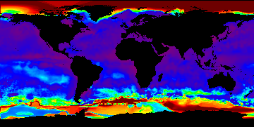
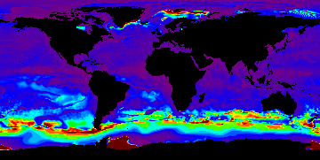
A few examples of the winter differences in the North Pacific are seen here: |
|
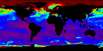
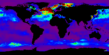
1999
February
|
TOPS ild
|
OTIS mld
|
|
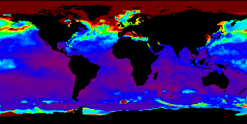
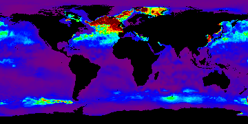
2000
February
|
TOPS ild
|
OTIS mld
|
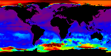
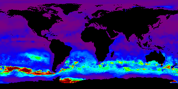
Differences in the Southern Ocean are more extreme:
|
1998
August
|
TOPS ild
|
OTIS mld
|
|
2002
October
|
TOPS ild
|
OTIS mld
|
last updated: November 15, 2006