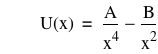
Phase-space trajectories for Lenard-Jones type Van der Waals potentials.
Version 0.2 2-5-10
To do:
(i) Refine considerably.
![]()
![]()
![]()
![]()
![]()
Morse-type potential.
![]()
![]()
![]()
![]()
![function(V,x)=V_0*[1-e^(-[x-a]/d)]^2-V_0](formula13.png)
![]()
![]()
![]()
![]()
![]()
![]()
![]()
![]()
![]()
![]()
Phase space trajectories associated with potential P. Mass and total energy.
![]()
![]()
![]()
![]()
![]()
![]()
Author: David A. Craig <http://web.lemoyne.edu/~craigda/>

This file was created by Graphing Calculator 3.5.
Visit Pacific Tech to download the helper application to view and edit these equations live.