3D dipole antenna pattern corresponding to simple linear antenna.
To do:
(i) Physically accurate field strengths
(ii) Solid angle slows things down considerably at higher resolutions...
Larmor formula: P=(2/3)(qa)^2/c^3; dP/d\Omega = (1/4pi)(qa)^2/c^3sin^2(theta).
![]()
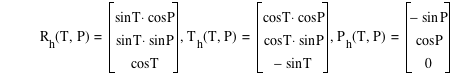
Acceleration of source charge:
![]()
![]()
![]()
![]()
![]()
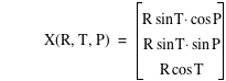
Electric field strength goes like (e/c)(a*sinT/r). (E is proportional to Xcross(Xcrossa).) Exhibit just angular dependence (f is a visibility scale factor):
![]()
![]()
![]()
Electric and magnetic field directions and Poynting vector (R,G,Y):
![]()
![]()
![]()
![]()
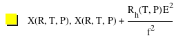
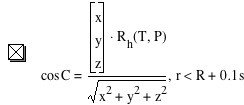
Solid angle around observation direction. (Higher resolution slows down plotting to a crawl, so don't try smaller opening angles at high resolution until observation direction has been set.)
![]()
![]()
Author: David A. Craig <http://web.lemoyne.edu/~craigda/>

This file was created by Graphing Calculator 3.5.
Visit Pacific Tech to download the helper application to view and edit these equations live.