Propagation of plane electromagnetic wave.

Version 0.4 12-3-06
To do:
(i) Fix Poynting vector
(ii) Plot just one plane of plane wave? (y=0 -like conditionals on plot command yield quirky results)


A – amplitude; K – wave number; W – (angular) frequency; c – wave speed

Maximum value of n should be a multiple of period 2pi/W so rollover in n is smooth.

A=1,K=pi,W=0.1*pi,c=W/K

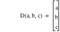
D – anchor point of field vectors;

function(D,a,b,c)=vector(a,b,c)

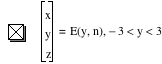
Electromagnetic wave propagating along y-axis; zoom -0.5<x,y,z<0.5 is nice:

function(E,s,N)=vector(0,0,A*sin([K*s-(W*N)])),function(B,s,N)=vector(A*sin([K*s-(W*N)]),0,0)

function(D,0,b,0),function(D,0,b,0)+function(E,b,n),in(b,set(-3,-2.9,-2.8,-2.7,-2.6,-2.5,-2.4,-2.3,-2.2,-2.1,-2,-1.9,-1.8,-1.7,-1.6,-1.5,-1.4,-1.3,-1.2,-1.1,-1,-0.9,-0.8,-0.7,-0.6,-0.5,-0.4,-0.3,-0.2,-0.1,0,0.1,0.2,0.3,0.4,0.5,0.6,0.7,0.8,0.9,1,1.1,1.2,1.3,1.4,1.5,1.6,1.7,1.8,1.9,2,2.1,2.2,2.3,2.4,2.5,2.6,2.7,2.8,2.9,3))

function(D,0,b,0),function(D,0,b,0)+function(B,b,n),in(b,set(-3,-2.9,-2.8,-2.7,-2.6,-2.5,-2.4,-2.3,-2.2,-2.1,-2,-1.9,-1.8,-1.7,-1.6,-1.5,-1.4,-1.3,-1.2,-1.1,-1,-0.9,-0.8,-0.7,-0.6,-0.5,-0.4,-0.3,-0.2,-0.1,0,0.1,0.2,0.3,0.4,0.5,0.6,0.7,0.8,0.9,1,1.1,1.2,1.3,1.4,1.5,1.6,1.7,1.8,1.9,2,2.1,2.2,2.3,2.4,2.5,2.6,2.7,2.8,2.9,3))

Poynting vector S; q scales it up a bit for visibility. S won't plot properly when hits end. (See below.) Not sure what's hinky.

function(S,s,N)=cross(function(E,s,N),function(B,s,N)*c/(4*pi))

q=slider([1,125])

function(D,0,5*b+c*n,0),function(D,0,5*b+c*n,0)+function(S,5*b+c*n,n)*q,in(b,set(-3,-2.9,-2.8,-2.7,-2.6,-2.5,-2.4,-2.3,-2.2,-2.1,-2,-1.9,-1.8,-1.7,-1.6,-1.5,-1.4,-1.3,-1.2,-1.1,-1,-0.9,-0.8,-0.7,-0.6,-0.5,-0.4,-0.3,-0.2,-0.1,0,0.1,0.2,0.3,0.4,0.5,0.6,0.7,0.8,0.9,1,1.1,1.2,1.3,1.4,1.5,1.6,1.7,1.8,1.9,2,2.1,2.2,2.3,2.4,2.5,2.6,2.7,2.8,2.9,3))

Works properly until g hits end of range – which may be related to the larger issue:

g=slider([-3,6])

function(D,0,g+c*n,0),function(D,0,g+c*n,0)+function(S,g+c*n,n)*q

Boundaries and interior of loops to assess curlE/B:

function(D,t*l,d,0)

function(D,l,d+t*l,0)

function(D,t*l,d+l,0)

function(D,0,d+t*l,0)

function(D,0,d,t*l)

function(D,0,d+t*l,l)

function(D,0,d+l,t*l)

d=slider([0,1])

l=slider([0,1])

function(D,u*l,d+v*l,0)

function(D,0,d+u*l,v*l)

Maxwell says that curlB=dE/dt and curlE=-dB/dt. Does our field agree?

View of full plane wave. Zoom of -1<x,y,z<1 is nice:

vector(x,y,z)=function(E,y,n),-3<y<3

vector(x,y,z)=function(B,y,n)

Use planes as shields to section plane wavefield:

x=h

y=j

z=k

h=slider([0,1])

j=slider([0,1])

k=slider([0,1])


Author: David A. Craig <http://web.lemoyne.edu/~craigda/>


Graph of the formula

This file was created by Graphing Calculator 3.5.
Visit Pacific Tech to download the helper application to view and edit these equations live.